I A Beginner’s Guided Tour
In this exercise, we will overview GrafEq’s functionality.
While the many screen-shots and pictures serve as a pleasant introduction to general users,
the step-by-step explanations will help the novice students follow through.
- For a general description for the GrafEq program, visit the on-line description page at
http://www.peda.com/grafeq/description.html.
- For an overview of the program’s functionalities, visit the on-line specifications page at
http://www.peda.com/grafeq/spec.html.
- This tutorial is based on GrafEq 2.05; users of other versions of GrafEq
might need to adjust some steps for any differences in the user interface.
I.1 Launch the program
- Double-click on the GrafEq icon, as seen in figure I.1 following:

Figure I.1: The GrafEq icon
- A splash screen appears, which gradually reveals the GrafEq title screen, as
seen in figure I.2 following. Press the space bar once to clarify the splash
screen and once more to remove it.

Figure I.2: The GrafEq title screen
- The Relation #1 algebraic window then opens automatically, as
seen in figure I.3 following:
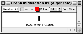
Figure I.3: An Algebraic Relation Window
I.2 Enter a relation
- Ensure that the caps lock key is not depressed.
- Follow the step sequence, which will be provided, to enter the relation
as seen in figure I.4 following:
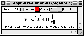
Figure I.4: y=sqrt(x)sin1/x
The necessary step sequence is as follows (Refer to the hints immediately
following regarding easy buttons and prompts.):
- Type in “y=”;
- Click the sqrt() easy button;
- Type in “x”, then “)”, noting the prompt at the bottom of
the relation window, that says “Press ) to finish the term”;
- Type in “sin1/x”.
Some general hints about entering relation specifications:
- Use the keyboard to enter letters, digits, brackets, and simple symbols such as
+, -, *, /, !, >, <, =, ...
- Use easy buttons
to enter special characters and
operators, such as algebraic powers and roots.
Figure I.5 following shows the easy button floating window:
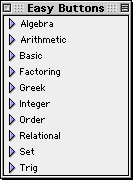
Figure I.5: Easy Button Floating Window
- The relation window also displays a prompt message to guide the user.
In an empty relation window, as in figure I.5, the help message prompts the user
to enter a relation.
Other appropriate messages appear at different stages of relation input.
- The relation window parses entries as a relation specification is being entered, and
displays them in standard mathematics format. The sequence of keyboard keys pressed
can be revealed by moving the cursor from the end of the entry line to the left.
- To make changes to the relation, or correct typing mistakes:
- position the cursor, with the mouse or the left and right arrow keys, to
where changes are to be made; (Any relation portions now behind the cursor
would become unformatted, as a sequence of keyboard entries;
don’t worry about them, they will become formatted again when
relation entry is completed, or when the cursor is placed back to the end
of the entry line.)
- press the delete key to erase the character
to the left of the cursor, and
press the del key to erase the character to the right of the cursor;
- The prompt message at the bottom of the window now states
“Press return to graph...”
Press return now. The Create View window will then appear.
Figure I.6 following is the create view window:
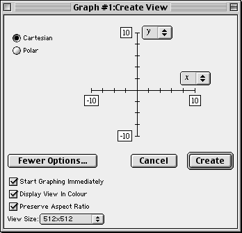
Figure I.6: The Create View Window
I.3 Specify a viewport
- GrafEq can plot both Cartesian and Polar graphs, and will automatically set
the default mode according to the relation entered.
The graph mode can be changed by clicking its radial button.
Since we have entered Relation #1 as a rectangular relation,
Cartesian mode is active (by default) in our Create View window, and we will not
change that.
- We will not change the default domain (horizontal) and range (vertical) bounds,
but any of them can be changed by:
- clicking on the box of the bound to be changed; then
- editing the number in the box; and
- repeating the steps for any other bounds to be changed.
I.4 Create a graph
- Create the specified view by clicking the Create button, or simply pressing return
as the Create button is the default button. (The thick border around the Create button
denotes that it is the default button.)
The graph view and an accompanying view buddy floating window appear as
in figure I.7 following:
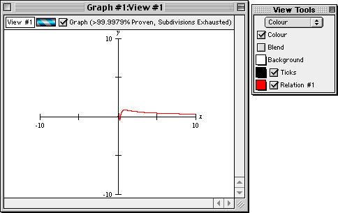
Figure I.7: Graph view of y=sqrt(x)sin1/x, and the view buddy
I.5 Apply and remove axes and scales
Figure I.7 shows axes and scales applied to the graph; the steps required to
remove or apply them are as follows:
- Go to the view buddy, click and hold down the mouse on the mode pop-up menu on the top
of the floating window; a pull down list appears.
- Drag the mouse down the list to Ticks, then release the mouse to enter Ticks mode.
- Click on each of the four buttons in turn to see the different ticks. Figure I.7
uses the second button.
- The Show Ticks checkbox on top of the buttons is selected. To hide the ticks,
click on the checkbox once to toggle ticks inactive. (One more click and
the ticks will be toggled active, into the last state selected.)
I.6 Alter the viewport region by zooming
The graph presents a good overview of the relation over the domain and range of
[-10, 10]. But the interesting portion seems to be a smaller region around the origin.
Although we could have created a view with narrower bounds in the Create View window,
it is now more convenient for us to change the viewport region with
GrafEq’s zoom feature.
- Return to the view buddy, and enter zoom mode by selecting
Zoom from the mode pop-up menu at the top of the floating window.
- The Zoom-Out button is on the view buddy now, but there is not a button for
zooming in, since we have to specify the region to be zoomed into.
- Place the mouse cursor within the graph view; a zoom box will appear.
- Place the zoom box at the graph’s interesting portion, close to the origin,
as seen in figure I.8 following:
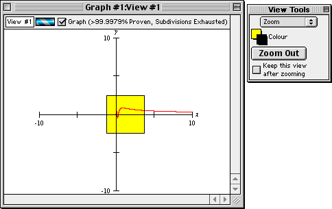
Figure I.8: Zooming into a graph's interesting area, with the zoom buddy
- Click once to see the selected region, as View #2.
- Zoom in to the center once again, to create View #3, as seen in figure I.9 following:
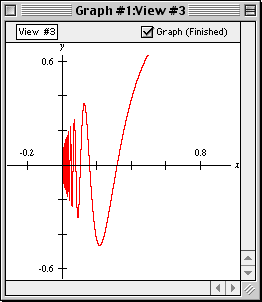
Figure I.9: A good view of the graph's interesting area
I.7 Edit a relation
We will edit the relation, from y=sqrt( x)sin1/ x to
y= x2sin x2.
- Bring the relation window back up front, to be the active window:
If some part of the window is visible, click on it once. Alternatively,
go to GrafEq’s top Graph menu, drag the mouse down to Relation #1(Algebraic), and
release the mouse to select the algebraic window for Relation #1.
| Hint: | The relation window appears, but not the prompt message
or the easy button floating window.
But the Active box in the relation window is selected, and
the graph of Relation #1 is shown in the View #3 window.
|
|
- Click once on the relation, to invoke its edit mode.
| Hint: | The prompt message appears in the relation window
and the easy button floating window appears next to the relation window.
But the Active box in the relation window is cleared, and
the graph of Relation #1 is not shown in the View #3 window.
|
|
- Place the cursor just in front of “sin”, as seen in figure I.10 following:
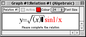
Figure I.10: Relation #1 being edited
| Tip: | Move the cursor by clicking the mouse in the area, or
by repeatedly pressing the left arrow key. |
|
| Hint: | The relation portion behind the cursor becomes unformatted.
Don’t worry about it; it will be automatically
reformatted as they pass to the left side of the cursor. |
|
- Erase the sqrt(x) term by either:
- highlight the term with the mouse and cursor, then press the del key, or
- press the delete key until the term is removed.
- Enter x2 as follows:
- Type in x from the keyboard;
- Go to the easy button floating window, and click the
arrow adjacent to the algebra easy button set to open it;
- Click the a2 button once, and the relation window will look
like figure I.11 following:
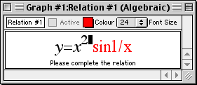
Figure I.11: Relation #1 edited
- Move the cursor to the rightmost end of the relation, and see that the entire
relation becomes formatted again, by:
- clicking the mouse there, or
- repeatedly pressing the right arrow key until the cursor is there, or
- holding down the control key and pressing the right arrow key once.
- Press the delete key three times to remove the 1/x term.
- Enter x2 one more time to complete relation editing, as
seen in figure I.12 following:
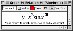
Figure I.12: Relation #1 edited
- Press return to see the new graph plotted in the View #3 window.
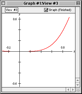
Figure I.13: Graph of the edited Relation #1
- The new graph above does not look very interesting. But note that the scales show very
small numbers, and remember that we had zoomed in twice to produce View #3;
we will now zoom back out to take a look at the “bigger picture”.
- Return to the zoom buddy, referring to the steps described earlier when altering
the viewport region, press the Zoom Out button a few times.
The result of zooming out is intriguing. The following picture, View #7, is
obtained after zooming out four times.
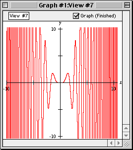
Figure I.14: Graph of the edited Relation #1 after four zoom-outs
I.8 Use constraints in defining a relation
Note that the graph in figure I.14 is much simpler where x is small
(less than three). We will now produce a simple graph whose domain is [0,3].
We have learned that:
- we can define the bounds in the Create View window, and that
- we can use the zoom feature of GrafEq.
Now we will use constraints in defining a relation.
- Bring the relation window back to the foremost and invoke its edit mode
(refer to the steps described earlier when editing a relation).
- The prompt message at the bottom of the window states “....press
tab to add a constraint.”. Press the tab key now.
- Enter the constraint “0<x<3”, as seen in figure I.15 following:
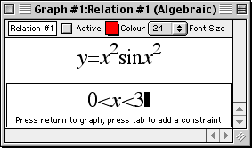
Figure I.15: Relation #1 with second constraint
- Press return for the resulting graph, as seen in figure I.16 following:
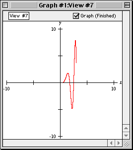
Figure I.16: Graph of Relation #1 with two constraints
Congratulations! You have completed the first part of this walk-through exercise!
Before you continue on to the next section of the exercise, it is good practice
to close your current graph, to free up the computer’s memory and screen space.
To close your graph:
- press the mouse button on the File menu, then
- drag the mouse down the pull-down menu to Close Graph, and
release the button to close your graph.
Graphs may also be saved, for future re-use. A later tour will discuss saving graphs
in the various formats supported by GrafEq.
In this section, we will try out graphing multiple relations on the same graph,
and a few other features of GrafEq.
I.9 Plot three simultaneous systems
- Under the File menu select New Graph, to get a new relation window.
- Enter Relation #1 as seen in figure I.17 following,
(with the help of the easy buttons for square operations):
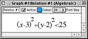
Figure I.17: Relation #1 for the simultaneous system
- Press return after Relation #1 is entered correctly, to get to
the Create View Window.
- The default settings are fine, so press return or click on Create to
create a graph.
- Under the Graph menu, select New Relation, to get another
relation window (entitled Relation #2).
- Enter the second relation,
referring to figure I.18 following, then press return.
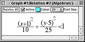
Figure I.18: Relation #2 for the simultaneous system
- Open another relation window (entitled Relation #3), by
selecting New Relation under the Graph menu.
- According to figure I.19 following, enter the first constraint of the relation, press Tab,
then enter the second constraint of the relation:
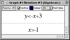
Figure I.19: Relation #3 for the simultaneous system
- Press return; your graph now shows all three relations in three different colours,
layered with Relation #1 at the bottom, then Relation #2, and finally Relation #3
on top, as seen in figure I.20 following:
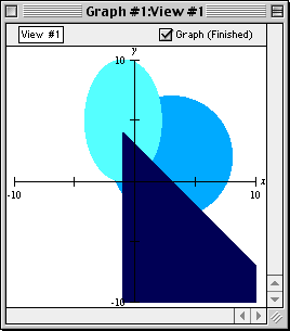
Figure I.20: Graph of the simultaneous system
I.10 Blend the graphs of three simultaneous systems
- Return to the view buddy, and return to colour mode by selecting
Colour from the mode pop-up menu on the top of the floating window.
- Click to select the Blend checkbox. The graphs for the simultaneous systems become
blended, revealing individual graphs and intersections of the simultaneous system,
as seen in figure I.21 following:
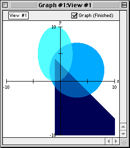
Figure I.21: Blended graph of the simultaneous system
I.11 Determine a point’s coordinates
- Return to the view buddy, and enter One Point mode by selecting
One Point from the mode pop-up menu on the top of the floating window.
- Place the mouse close to an intersection point on the graph; pin down the point
with the help of the magnified view on the view buddy, as seen following:
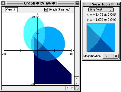
Figure I.22: Pin down an intersection point with the one point view buddy
- Read the coordinates of the point from the view buddy.
I.12 Change the colours of the graphs
- Access the colour mode view buddy again.
- Click on the colour box of Relation #1. When the colour panel appears, drag the
highlight box to choose another colour.
- Repeat the process to choose colours for any other relations.
I.13 Determine the distances between points
- Access the Two Point mode of the view buddy. A line segment AB appears
on the graph.
- Use the mouse to drag points A and B to the two ends of the distance to be measured.
See figure I.23 following as an example:
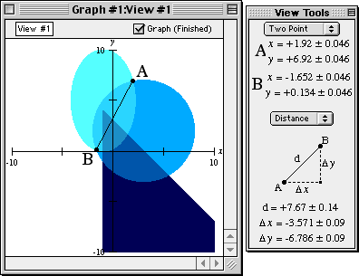
Figure I.23: Measure distance between two points with the two point view buddy
- Read the distances from the view buddy.
Congratulations! You have completed this introductory tour
and experienced the basics of GrafEq.
As a reward for completing the tour, graph the relation in figure I.24 following:
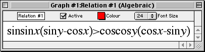
Figure I.24: Reward Relation
Many other features remain to be explored, such as:
- copying and pasting relations and graphs,
- making pages for printing,
- saving graphs to disk,
- using custom ticks,
- using one-key short-cuts, and
- customizing GrafEq for subsequent sessions.
Refer to the manual for full details of GrafEq’s functionality;
the appendices provide a useful summary and reference.
Pedagoguery Software will be placing additional tours online at
http://www.peda.com/grafeq/tutorials.html,
and with the manual.
|
|